James Bryant Consultant Engineer - Analog Electronics
RTFDS-2
Operational Amplifier Noise
This one of a series of short articles on problems in analog electronics which can be better understood by an enlightened study of the data sheet concerned.
Noise has two different meanings: it can mean an external signal which finds its way, unwanted, into a circuit or system (summarised succinctly, if not quite accurately, as "a wanted signal in a place you don’t want it"), or it can mean a random signal generated within a circuit or system by physical processes within that circuit or system which are not connected with the signal(s) that that circuit is supposed to be handling. It is the latter variety that we shall be discussing in this article.
Before discussing the noise in operational amplifiers it is well to define a few terms. In fact we shall spend almost half of the article in defining terms, and the terms so defined will be of value in any study of noise in electronic systems, not just the noise of op amps.
Noise is, as we have already stated, a random signal generated within a circuit of system by physical process within that system. If a noise source generates noise at all frequencies, and the amount of energy in a given bandwidth is unaffected by the centre frequency (e.g. the noise energy in the band 9-11Hz is the same as in the bands 999-1,001Hz or 999,999-1,000,001Hz) then the noise is said to be white noise and its noise spectral density is constant with frequency. In practice no noise source is white from DC to infinity and the term white noise is commonly used of noise whose noise spectral density is constant over some band of interest.
The term noise spectral density describes the power within a given bandwidth. It is occasionally expressed in terms of power - Watts/Hertz (more practically in real systems as pW/Hz or fW/Hz or even aW/Hz) but is far more commonly specified in voltage or current. For a given resistance power is proportional to the square root of voltage (or current). Therefore when, as is usual, noise spectral density is given in terms of voltage or current, rather than power, the units become V/√Hz or A/√Hz (or again, more practically, nV/√Hz or pA/√Hz).
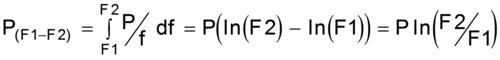
By analogy with white noise, pink noise is noise where the noise spectral density is higher at low frequencies. Its commonest form is 1/f noise, where the (power) noise spectral density is inversely proportional to frequency. Working in voltage (or current) this is, of course 1/√f noise, but the term 1/f noise is still generally used for it. At very low frequencies below a µHz (1µHz is one cycle every 11½ days) the 1/f law breaks down but it is reliable at quite low frequencies. Intuitively one might expect noise power to rise dramatically at very low frequencies (it would, after all, be infinite at DC if the law survived that far). In fact it rises, but not dramatically. If we have a 1/f noise source with a power noise spectral density of P/Hz at 1 Hz we can calculate the total power between any two frequencies F1 and F2 (F2>F1) where the 1/F law applies by evaluating the integral
[1]
If we transform this for the case where the voltage noise spectral density is V/√Hz at 1Hz we find that the total r.m.s. voltage noise V(F1-F2) between F1 and F2 is given by
[2]
It is obvious that [1] & [2] blow up on us at DC (ln(0) = -∞) but we can solve for F1 = 1Hz and F2 = 2Hz
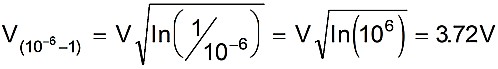
We can also solve it for F1 = 1µHz and F2 = 1Hz
From which we see that the power in the band 1µHz - 1Hz is about 20 times the power in the band 1-2 Hz, and the rms noise voltage is about 4.5 times as large. This is not so terrifying.
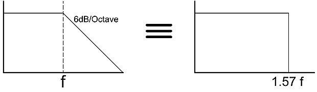
When we discuss noise in a bandwidth F1-F2 the basic mathematics assumes that all the noise below F2 is present, and all the noise above F2 is filtered. Real analog filters do not behave like that. If we filter noise in a single pole low pass filter with a “cutoff frequency” of F the 6dB/octave rolloff means that the total rms noise in the filter output will be the same as the rms noise we would expect from a sharp cutoff filter at 1.57F. The equivalent figure for a two pole filter is 1.2F.
Fig. 1. Single Pole Filter - Power in Stop Band.
When IC op amps were first developed the most important noise specification was popcorn noise which was so called because, played through a loudspeaker, it sounded like cooking popcorn. It consists of random step changes of Vos in a timeframe of 100mS - 10S. Popcorn noise is the result of imperfections in IC processing and today the mechanisms involved in causing popcorn noise are better understood. Op amp manufacturers not only take precautions to minimise popcorn noise, but when it does occur at a significant level it is recognised and the devices concerned are scrapped. It is unlikely that it will ever be eliminated completely, but with the precautions and testing mentioned above it has ceased to be a major problem and is now merely a minor nuisance. Today popcorn noise is not specified separately in most devices but forms a relatively minor component of the 1/f noise we have just discussed.
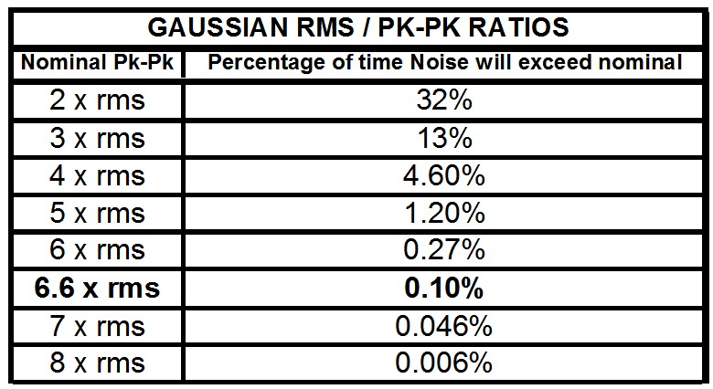
Noise in op amps is Gaussian (or if it not Gaussian it is so close to Gaussian that several decades of research have been unable to prove it is not). It is a feature of Gaussian noise that the probability of a particular noise amplitude being exceeded diminishes as the amplitude increases - but the probability never becomes zero. A mathematician would say that it is therefore meaningless to refer to peak noise in a Gaussian system - if we wait long enough whatever peak we have chosen will be exceeded. The table in Fig. 2 shows the relationship between peak peak and rms values in a Gaussian system.
Fig. 2. Gaussian r.m.s. / pk-pk Ratios.
The majority of readers of this article are engineers, not mathematicians, and are prepared to be slightly less rigorous. While it is clearly better to define rms noise since that is more rigorous, it is possible to define peak-peak noise if we include in our definition some specification of how often it will be exceeded. The commonest convention is <0.1% of the time, which corresponds to a pk-pk value 6.6 times the rms value. What we must not do is define peak noise without this qualification, since all devices will be out of specification according to such a definition.
If the same noise (with or without sign change) appears at two or more points in a circuit the two noise sources are said to be correlated. More commonly if two noise sources are completely independent they are said to be uncorrelated. Sometimes, when the noise at each of two (or more) nodes is derived from several different sources and some of the sources are identical the noise is said to be partially correlated. For practical purposes correlation of lest than 10-15% can usually be disregarded.
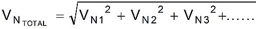
Since noise powers add, uncorrelated noise voltages or currents are added as the root sum of squares:-
[3]
It is evident from this that if a single term is less than 20% of some other term in the total it can generally be disregarded as making little contribution to the total noise. Of course if there are very large numbers of small terms the analysis is more complex. Correlated noise signals are just added.
All resistors have Johnson Noise or thermal noise. This is implicit in the physics of resistance, and is not an imperfection. (Reactances - capacitors and inductors - do not have Johnson Noise, except the Johnson Noise of any parasitic resistance.) Of course some types of resistor (especially very high value ones) may have higher levels of noise than the Johnson Noise, and the noise of some resistors may vary with current flow. These are imperfections, but the basic Johnson Noise of √4KTR V/√Hzis intrinsic to any resistor. Today, in fact, the noise of most (but not all) types of resistor is quite close to their theoretical Johnson Noise. We can reduce T, the Kelvin temperature (but note that cooling to liquid nitrogen temperature of 77K is needed to reduce the noise voltage by 50%) and we can reduce the resistance, R, but we cannot reduce Boltzmann’s Constant, k (= 1.38x10⁻²³ Joules/K), because Boltzmann has been dead since 1906.
When a current flows in a conductor or a resistor (the two are essentially the same) the charge moves as an “electron cloud” where charge carriers are not clearly associated with any one atom. However, when a current flows across a junction in a semiconductor (or, indeed, between the anode and cathode of a tube - which was where the effect was first noticed) the current is carried by discrete charge carriers, electrons (or holes), in discrete packets. These carriers behave in a statistical manner and current across a junction has intrinsic Shottky noise or shot noise of √2qIj A/√Hz where Ij is the junction current and q is the charge of an electron (1.6x10⁻¹⁹ Coulombs). Since the shot noise is proportional to the square root of the junction current it follows that although the noise rises as the current increases the noise as a percentage of the total current falls with increasing current.
The noise gain of an op amp is the voltage gain seen by the voltage noise of the amplifier, which is not necessarily the same as the signal gain. It may be thought of as the reciprocal of the feedback attenuation and is useful when calculating the noise of a circuit, but is even more important when calculating the stability of uncompensated op amps, an issue which is outside the scope of this article.
The final term that we shall define should rarely, if ever, be used in connection with op amps. The noise figure of an amplifier or other device is defined as the ratio of the noise of the device used with a particular source impedance relative to the noise of a perfect noise free device used in the same way. This is a very useful concept in RF, video and telephony where the majority of systems work with defined resistive sources and loads of 50Ω, 75Ω and 600Ω respectively, but is essentially useless with op amps which are used in a wide variety of different environments. It is meaningless to ask for the noise figure of an op amp in the abstract - it is only useful to ask for the noise figure in a particular application. The very act of asking for the noise figure of an op amp betrays ignorance of the nature of a noise figure, and of the way op amps are used.
For practical purposes an op amp can be considered as a noise free op amp plus three uncorrelated noise sources: a voltage noise source applied differentially between the two inputs and two current noise sources, one in series with each input. In fact the two current noise sources may have some degree of correlation but it is sufficiently small that for practical purposes they may be considered uncorrelated. Fig. 3A shows a model of the voltage noise source, Fig. 3B shows one of the current noise sources.
Fig. 3. Op-amp Voltage & Current Noise Models.
Both the voltage and current noise are white over much of the operating frequency range of the op amp, but at low frequencies they start to rise with the 1/f characteristic we discussed above. The transition frequency at which the plot of the noise spectral density v frequency changes from 1/f to white behaviour is known as the 1/f corner frequency and is a figure of merit for the amplifier, the lower the better. The voltage noise of a very low noise op amp may have a 1/f corner as low as a few Hz, general purpose op-amps are likely to have one of 20-100Hz, and high speed op amps may have it as high as 1-2KHz. (High speed op amp processes are optimised for speed rather than low frequency noise - the two being, to a certain extent, mutually exclusive.) The 1/f corner frequency for the voltage noise is not necessarily the same as the 1/f corner for the current noise - either may be the higher.
The voltage noise always appears at the op amp output. The current noise generates a voltage when it flows in the impedance present on the input. Therefore the current noise is unimportant if the impedance at the input nodes is low enough. We shall discuss this a little later.
The range of voltage noise is not very wide. In general, conventional bipolar junction transistor (BJT) op amps and transimpedance (current feedback) op amps have good voltage noise but poor current noise, while BIFET amplifiers have good current noise and poor voltage noise. (Most CMOS processes make op amps with very poor voltage noise but it is not intrinsic to all CMOS processes and amplifier CMOS processes exist with reasonable amplifier voltage noise.) BIFET op amps (AD743 & AD745 are examples) have been designed with very low voltage noise as well as extremely low current noise. The problem with such amplifiers is that the large JFETs in their input stages, which are necessary for the low noise, have quite a large capacitance, which complicates the circuitry in which they are used.
The very best low noise op amps have noise spectral density as low as 0.6nV/√Hz at mid frequencies (equivalent to the Johnson Noise of a 22Ω resistor at 25°C) and few, if any, are worse than 15nV/√Hz. The voltage noise spectral density is, as I have said, normally specified at mid frequency and it is usual for it to be flat from the 1/f corner to well above the unity gain frequency. If for any reason the noise spectral density does vary with rising frequency a plot of noise v frequency will probably be included in the data sheet.
The 1/f corner may be anywhere between 2Hz and 2KHz. It will generally be specified, but if it is not the data sheet may contain details of noise spectral density at 10Hz or the total noise voltage in the range 0.1-10Hz. Provided that the 1/f corner frequency is above 10Hz it is possible to calculate the 1/f corner frequency from this data.
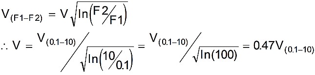
If we do not have the spectral density at some frequency within the 1/f region we can can calculate one using the integral from Equation [2] above. The rms noise voltage between F1 and F2 (where F2 is still in the 1/f range) for noise which has a spectral density of V at 1 Hz is V√ln(F2/F1)
If we know the rms noise voltage, V(F1-F2), in the band F1=0.1Hz and F2=10Hz, we can solve for V:
[4]
which gives us the voltage noise spectral density at 1Hz. We can use this value in the next part of the calculation. If, of course, the data sheet gives us a spectral density in the 1/f region we do not need the calculation above but can go there directly.
If the mid band spectral density is X1 and the spectral density at FHz within the 1/f region is X2 (the figure is usually given at 10Hz on data sheets, but let’s take the general case, especially as the value calculated in [4] above was for 1Hz) then the 1/f corner frequency Fc is given by:-
[5]
Current noise flows in both the inverting and non inverting inputs of the op amp and In+ and In- are effectively uncorrelated. In conventional (voltage feedback) op-amps In+ and In- are approximately equal in amplitude, though uncorrelated, but transimpedance (current feedback) op amps, which have different structures in their inverting and non inverting inputs, have completely unmatched In+ and In- with different magnitudes, different TCs and even different 1/f corner frequencies.
Op amps can have a much wider range of noise currents than noise voltages. The AD549 has current noise of 140aA/√Hz (= 0.14fA/√Hz) while the AD9617 has current noise of 30pA/√Hz, a factor of over 200,000 times greater. It is common to find that data sheets do not specify the noise current of op amps. Where op amps have simple BJT or FET input stages their current noise is simply the shot noise of their bias current and may therefore be calculated from the bias current, Ib, and q, the electron charge (1.6x10⁻¹⁹ Coulomb).
In = √2qIb A/√Hz
Transimpedance op amps and bias compensated op amps such as the OP 07 have much greater noise current than the shot noise of their bias current. This is because their bias current is the difference current between two much larger, and approximately equal, currents flowing within the device. Since the noise on these two currents is uncorrelated the external noise current is the rms sum of the two. It cannot be predicted from their bias current - all that can be said is that it will be much larger than the shot noise of the bias current.
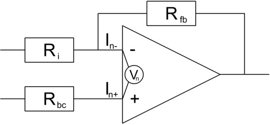
To end this review of op-amp noise let us consider the typical op-application circuit shown in Fig. 4. To assess the noise of this circuit we must calculate the effect on the noise spectral density at the output of six different noise sources:-
[1] Johnson noise in Ri = √4kTRi (Rfb/Ri); [2] Johnson noise in Rbc = √4kTRbc (Rfb/Ri); [3] Johnson noise in Rfb = √4kTRfb; [4] Amplifier voltage noise = Vn(1+Rfb/Ri); [5] Amplifier current noise (inverting IP) = In-Rfb; and [6] Amplifier current noise (non-inv IP) = In+Rbc(1+RIn-Rfb/RIn-Ri)
The total noise of all of these sources is
In a practical design it is necessary to evaluate each term in the expression above. Almost always some terms will be found which are much smaller than others - any term which is smaller than 1/5 of any other can be disregarded (even if five terms are equal and each is 1/5 of the sixth term they will all make under 10% difference to the final value).
Evaluating this expression with different values of Vn, In and resistance shows that with low resistance the voltage noise of the amplifier is dominant, and at high enough resistance the current noise of the amplifier, no matter how low, will dominate. There is a region between, though, where the Johnson Noise of the resistors may be dominant if the current noise is low enough - if the current noise is large, though, the transition may be directly from voltage to current noise domination as resistance is increased, without a Johnson Noise region.
We thus see that in some circumstances (low impedance) we should choose an op-amp with low voltage noise and disregard its current noise. In others (very high impedance) we can disregard voltage noise and worry only about current noise. But there is a wide middle ground where the intelligent designer will carefully trade off voltage noise, current noise, and the Johnson Noise of his resistors to achieve minimum system noise.
The circuit in Fig. 3 shows only resistances. In many applications there may also be reactances (capacitors and inductors) in the system. These do not contribute noise, but if noise current flows in a reactance there will be a voltage, and of course they will affect system gain and frequency response. The analysis is similar to the resistive case we have studied but somewhat more complex.
Newbury - England 1995-08-05
Revised 2015-10-10
[Note that although this has been revised, many of the examples still date back 20 years to the original article.]
 [1]
[1]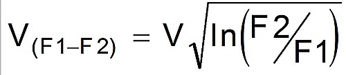 [2]
[2]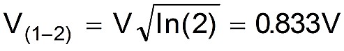
 [3]
[3]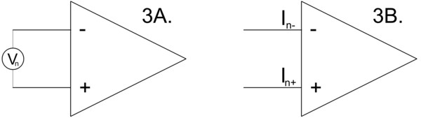
 [4]
[4]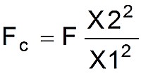 [5]
[5]